Naive Bayes - Supervised Learning Classification
AI Series - Chapter 6

I am a software engineer.
print("Naive Bayes")
Naive Bayes(NB) is a supervised learning model used for classification tasks. NB makes predictions by calculating the probability of event A happening given that B happened.
To understand NB we need to first understand conditional probability and Bayes Rule. Our prior knowledge of Precision and Recall would come in handy here. So I believe we can remember True Positives, True Negatives, False Positives, and False Negatives 👽.
Let's start with an illustration once more 😶.
Consider this made-up lab test result of people for COVID:
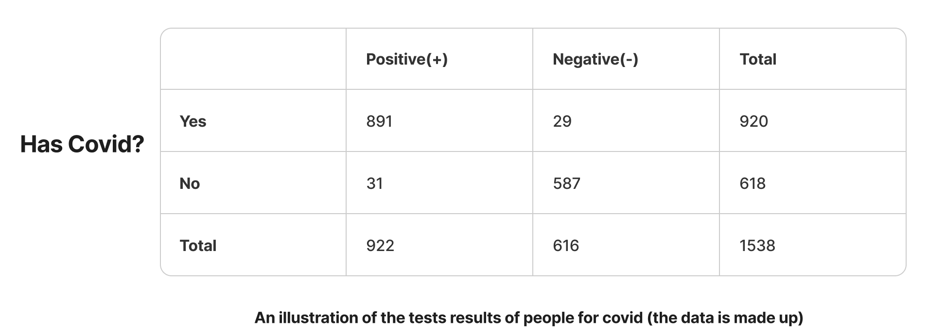
From the results table above we can deduce the following;
True Positives - The number of people that tested positive and actually had COVID = 891
False Positives - The number of people who tested positive but did not have COVID = 31
False Negatives - The number of people who tested negative but actually had COVID = 29
True Negatives - The number of people that tested negative and did not have COVID = 587
With this precedent, let's try to determine the conditional probability. Let's say we want to determine the probability of having COVID given that you tested positive;
We can use this simple formula:
Probability of A given B = tested positive/ total positive test
P = 891/922 = 0.9663 = 96.63%
Thus (ancient word lol), the probability of having COVID given that you tested positive is 96.63% using our made-up data.
So now let's talk about Bayes Rule.

Bayes Rule
Bayes Rule is the probability of an event A happening given that B happened.
The formula:
P(A|B) = P(B|A) * P(A) / P(B)
This means:
P(A|B) = Probability of A given B
P(B|A) = Probability of B given A
P(A) = Probability of A
P(B) = Probability of B
This means we can find the probability of P(A|B), as long as we know the probability of P(B|A), P(A), and P(B).
Example
Consider a problem given to us to calculate the probability of a person having COVID and testing positive, given that:
P(false positive) = 0.15
P(false negative) = 0.05
P(COVID) = 0.1
P(COVID/+) = ? (Probability of having COVID given that you tested positive)
Using our Bayes Rule:
P(COVID/+) = P(+/COVID) * P(COVID) / P(+)
P(+/COVID) = 1 - P(false negative) = 1 - 0.05 = 0.95
The above means the reciprocal of P(false negative) is equal to P(+/COVID)
P(COVID) = 0.1
P(+) = P(+/COVID) * P(COVID) + P(+/ No COVID) * P(No COVID)
\= (0.95 0.1) + (0.15 * 0.9) = 0.23
Where P(No COVID) = Reciprocal of P(COVID) = 1 - 0.1 = 0.9
Therefore:
P(COVID/+) = 0.95 * 0.1 / 0.23 = 0.413
Finally, we've concluded that the probability of having COVID given that you tested positive given our problem above is 0.4 or 40%.
Whew that was a lot right? 🥲
Now let's talk about the Naive Bayes rule.

Naive Bayes Rule
The Naive Bayes Rule in classification tasks calculates the probability of a class (Ck) given some feature vectors (x) using Bayes' theorem. This is based on the Bayes rule.
The formula:
P(Ck|x) = P(x|Ck) * P(Ck) / P(x)
This means:
P(Ck|x) = The posterior probability of class Ck given feature vector x.
P(x|Ck) = The likelihood of observing feature vector x given class Ck.
P(Ck) = The prior probability of class Ck.
P(x) = The probability of observing feature vector x. Also called the evidence.
The point of this being naive is that it makes a simplifying assumption that the features in a dataset are independent of each other, which may not always be true in practice.
Consider the dataset table below classifying a fruit as either orange or banana based on two features: color (orange or yellow) and shape (round or curved):
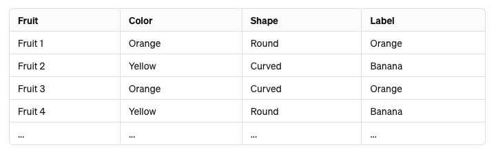
We can first observe that in this dataset the color and shape of a fruit are not independent. But in Naive Bayes, each feature we see, color and shape is treated as independent of any other feature.
That is why it is called "naive" because it makes such an assumption. Despite that, it works pretty well in classification tasks.
Playground
Remember our playground website? https://retzam-ai.vercel.app. For this chapter, we trained a model to predict whether a football player would get injured in their next football match using the Naive Bayes model. You can go and try it out directly here.
Enter the player's details as shown below.
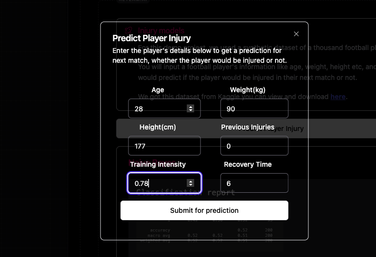
The model would predict if the player would be injured or not as shown below. It also shows the classification report of the model, so we can determine and assess its performance.
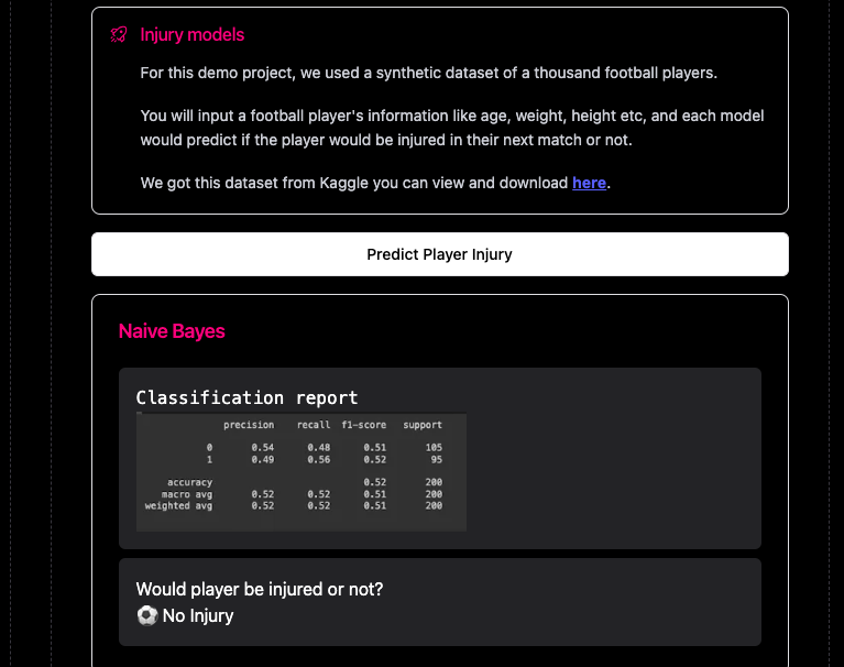
We also have a K-Nearest Neighbor model doing the same thing as well, so you can compare the prediction of both models. KNN might say the player would be injured while Naive Bayes would say the player won't be injured 🙂.
The rest of this chapter is optional for those who want to see how it is implemented hands-on. I recommend it for everyone though. If not you can skip to the end 🙂.
Hands-On
We'll use Python for the hands-on section, so you'll need to have a little bit of Python programming experience. If you are not too familiar with Python, still try, the comments are very explicit and detailed.
We'll use Google Co-laboratory as our code editor, it is easy to use and requires zero setup. Here is an article to get started.
Here is a link to our organization on GitHub, https://github.com/retzam-ai, you can find the code for all the models and projects we work on. We are excited to see you contribute to our project repositories 🤗.
For this demo project, we'll use a synthetic dataset of a thousand football players from Kaggle here, to help us predict if a football player would get injured or not. We'll use the Naive Bayes model.
For the complete code for this tutorial check this pdf here.
Data Preprocessing
Create a new Colab notebook.
Go to Kaggle here, to download the players' injury dataset.
Import the dataset to the project folder
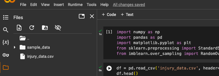
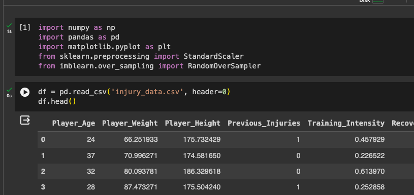
Import the dataset using pandas
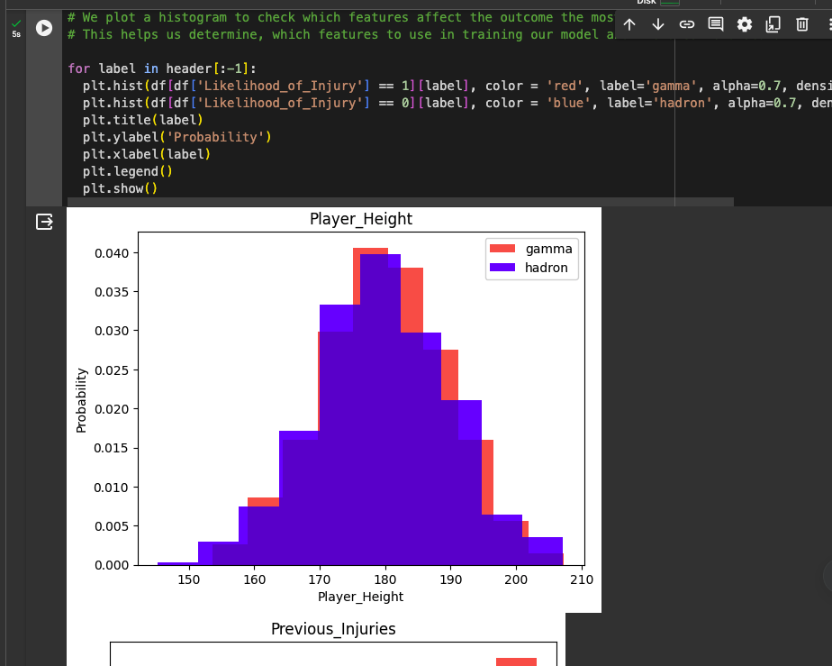
We plot a histogram to check which features affect the outcome the most or the least. This helps us determine, which features to use in training our model and the ones to discard.
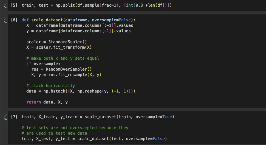
We then split our dataset into training and test sets in an 80%-20% format.
We then scale the dataset. X_train is the feature vectors, and y_train is the output or outcome. The scale_dataset function over samples and scales the dataset. The pdf document has detailed comments on each line.
Train model
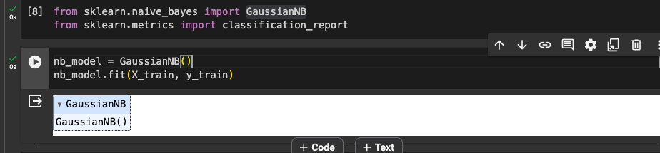
We don't need to create our Naive Bayes classifier from the bottom up by ourselves we'll use a library that already implements it from Scikit-learn: GaussianNB (Gaussian Naive Bayes). So we'll import it and train our model with our training dataset.
Performance Review
First, we'll need to make predictions with our newly trained model using our test dataset.
Then we'll use the prediction to compare with the actual output/target on the test dataset to measure the performance of our model.
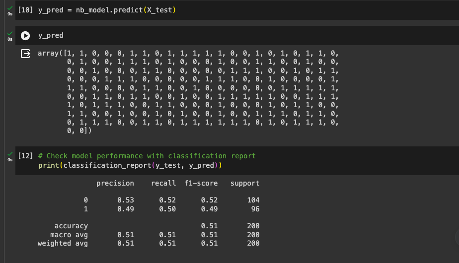
We can see our classification report, 51% accuracy is not good, right? Well yes. We can make this better by removing some features and making some adjustments. Training AI models is an iterative task.
Sometimes the model type doesn't suit the dataset. So a dataset might be better for a KNN model while another might have a higher accuracy using a Naive Bayes model.
Check the playground and compare the model's classification reports and predictions.
End of hands-on
So that's that about Naive Bayes 🤝, hope you learned something this week 👽. Don't forget to practice and use the playground and code base to help you grow.
Our next model is Logistic Regression, believe it or not, it is a classification model despite the "regression" name. We'll train a model to do something cool yet again, so stay tuned 🤖.